Affordable Computer Vision: A Myth No More

By: Valerii Haidarzhy, 21 Mar 2024

17 minutes

Reading Time: 17 minutes

Today, there are constant continuous battles on the Internet about whether it makes sense to invest money in a skilled team to create your own CV solution. It’s a never-ending debate, where supporters often mention the success of custom-designed systems for specific needs, like enhancing product quality control or improving analytic systems. Detractors highlight the high costs and complexities involved, especially the fear of needing top-tier, expensive hardware. However, our internal research challenges this concern. We’ve found that creating tailored solutions doesn’t always mean breaking the bank on hardware. Using cost-effective components and efficient coding, Mykhailo Koiev, our embedded engineer, has led our team to significant results. Now, let’s take a look at the process from the inside.

Choosing Hardware

“The combination of its relatively low cost, accessibility, and efficient hardware functionality for neural network operations makes this single-board computer highly attractive. Users can configure a neural network for specific tasks by leveraging libraries such as TensorFlow and effectively process input data. It’s important to note, however, that initializing the accelerator for a particular task requires some time.”
© Mykhailo Koiev, Embedded engineer, Sirin Software

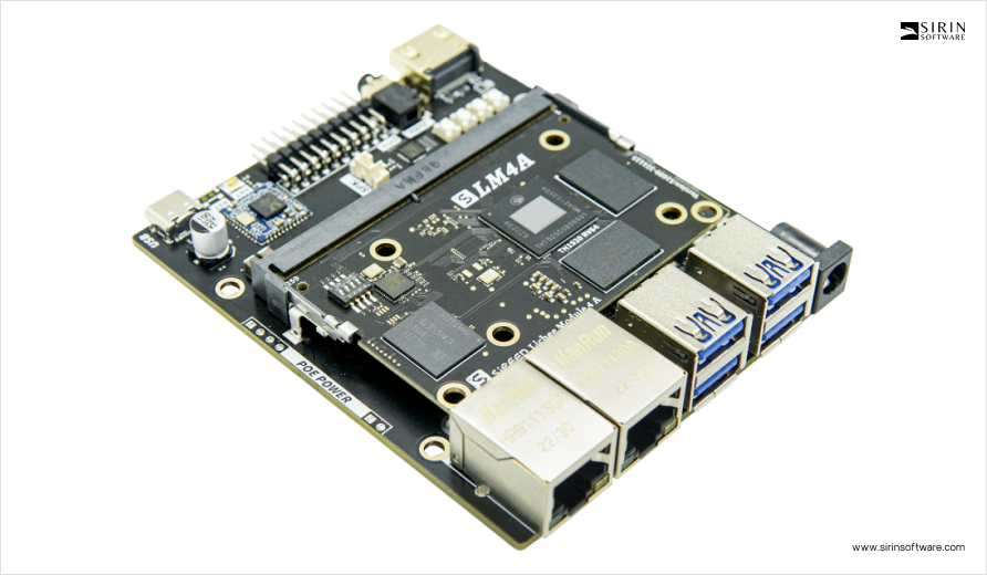
Scalability and cost-effectiveness, which are the main concerns for those who don’t believe in effective custom CV solutions, are two sides of the same coin. We had to look across devices, serving not just the high-end market but also more modest setups. This universality is achievable but only possible with a keen eye on optimization. And when it comes to costs, splurging on high-end hardware as a workaround for inefficiency is unsustainable. After considering everything, to explore CV applications, we settled on the LicheePi 4A Module, primarily because of its NPU* capabilities.

While banking on its mix of flexibility and strength that makes this SBC suitable for various uses, we had some concerns. The board’s software support could be limited, which might challenge specific applications. Additionally, while it offers robust capabilities, it couldn’t always match the raw power of some higher-end single-board computers available today. Below, we will describe the entire development path that our team has gone through to answer these concerns.

* A Neural Processing Unit (NPU) – specialized hardware accelerator designed for the efficient execution of neural network-based computations, particularly for machine learning and artificial intelligence tasks. Unlike general-purpose CPUs (Central Processing Units) or GPUs (Graphics Processing Units), NPUs are oexplicitly optimizedfor the parallel processing and computational patterns involved in neural network inference.

Software environment

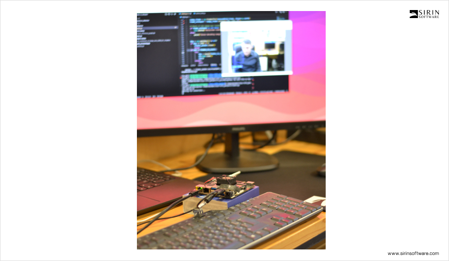
We started with preparing and installing the necessary software environment on the LicheePi 4A board and deploying it into a Docker container on the host machine. Since the board was new, we followed specific instructions to flash it, preparing it with the Debian GNU/Linux 12 (bookworm) operating system. This OS choice was deliberate, given Debian’s stability and extensive package repository, which, in our case, is ideal for development and research.

In our case, the board has OS:

sipeed@lpi4a:~$ cat /etc/os-release PRETTY_NAME=”Debian GNU/Linux 12 (bookworm)” NAME=”Debian GNU/Linux” VERSION_ID=”12″ VERSION=”12 (bookworm)” VERSION_CODENAME=bookworm ID=debian

Python Environment Configuration

With Debian installed, we made sure that Python version 3.11 was pre-installed on the system right after we burn LPi4A onto it.

It can be confirmed with the following command:

python –version

Most of the packages that the various Python programs depend on can be installed via pip, which can be installed with the following command:

apt install python3-pip

Pip acts as a gateway to a repository of Python packages, making it straightforward to install additional libraries and tools.Before installing other Python packages, the ‘venv’ package was installed, which is used to create a Python virtual environment:

apt install python3.11-venv

We then proceeded to install pip using apt install python3-pip and set up a Python virtual environment with apt install python3.11-venv.

A Python virtual environment was created and activated as follows:

cd /root python3 -m venv ort source /root/ort/bin/activate

to manage dependencies effectively and avoid conflicts between projects.

Preparation of NPU Environment

To utilize the NPU, we installed the shl-python library with ‘pip3 install shl-python‘, and copied the *.so files of the installed package to /usr/lib, enabling the shl-python library to interact with the NPU for hardware-accelerated neural network computations.

The shl-python library was installed using:

pip3 install shl-python

The location of the *.so files was identified with:

(cv_prj) sipeed@lpi4a:~$ python3 -m shl –whereis th1520

This command revealed the files at

/home/sipeed/prj/test/cv_prj/lib/python3.11/site-packages/shl/install_nn2/th1520

Then, the files were copied:

(cv_prj) sipeed@lpi4a:~$ sudo cp /home/sipeed/prj/test/cv_prj/lib/python3.11/site-packages/shl/install_nn2/th1520/lib/* /usr/lib/

Installation of HHB-onnxruntime

This stage was needed to confirm that our system could handle advanced computational tasks efficiently. HHB-onnxruntime is a component that allowed us to integrate the SHL backend (execution providers) with onnxruntime. It is significant as it enables onnxruntime to leverage the high-performance optimized code within SHL, for efficient execution of operations on both the CPU and NPU.

For the CPU setup, we used the following commands to download and install the necessary wheel file:

wget https://github.com/zhangwm-pt/onnxruntime/releases/download/riscv_whl_v2.6.0/hhb_onnxruntime_c920-2.6.0-cp311-cp311-linux_riscv64.whl pip install hhb_onnxruntime_c920-2.6.0-cp311-cp311-linux_riscv64.whl

Similarly, for the NPU setup:

wget https://github.com/zhangwm-pt/onnxruntime/releases/download/riscv_whl_v2.6.0/hhb_onnxruntime_th1520-2.6.0-cp311-cp311-linux_riscv64.whl pip install hhb_onnxruntime_th1520-2.6.0-cp311-cp311-linux_riscv64.whl

Next, we focused on installing libraries for our Python environment: openCV and numpy. These libraries provide functionalities for image/video processing and data array manipulation.

We opted for precompiled versions of these libraries for our setup process:

# Clone the prebuilt_whl repository and navigate to the directory git clone -b python3.11 https://github.com/zhangwm-pt/prebuilt_whl.git cd prebuilt_whl # Install the precompiled numpy and openCV libraries for Python pip install numpy-1.25.0-cp311-cp311-linux_riscv64.whl pip install opencv_python-4.5.4+4cd224d-cp311-cp311-linux_riscv64.whl

And our system was equipped with the necessary tools for advanced computation.

Notes: HHB provides the tools to compile neural network models for various hardware accelerators, including GPUs and TPUs. The process involves converting a neural network model into a common intermediate format, such as ONNX, Keras, or TensorFlow, which is then used to generate executable code for specific hardware accelerators.

Host actions

Here, we concentrated on model conversion and compilation, utilizing a Docker container. Docker’s ability to encapsulate environments makes it an ideal choice for consistency across different platforms. Here’s how we executed this step:

We began by pulling the necessary Docker container using:

docker pull hhb4tools/hhb:2.4.5

Next, we ran the Docker container in detached mode, naming it ‘your.hhb2.4’ and mapping port 22 to maintain access to the container:

docker run -itd --name=your.hhb2.4 -p22 hhb4tools/hhb:2.4.5

To perform operations within the container, we executed an interactive bash shell:

docker exec -it your.hhb2.4 /bin/bash

And then set the PATH variable to include the Xuantie-900 toolchain for our compilation tasks:

export PATH=/tools/Xuantie-900-gcc-linux-5.10.4-glibc-x86_64-V2.6.1-light.1/bin/:$PATH

Finally, we verified the availability of the HHB tools by checking the version:

hhb --version

Clone and convert Yolov5n to ONNX format

To optimize the model’s compatibility with our environment, we had to convert the YOLOv5n model to ONNX format.

We cloned the YOLOv5 repository, using the branch tagged as v6.2, to confirm we were using the correct version of the model for our needs:

git clone https://github.com/ultralytics/yolov5.git

cd yolov5

And installed the Ultralytics library, which provides tools for working with computer vision models:

pip3 install ultralytics

Lastly, executed the export script to convert the Yolov5n model weights to the ONNX format, specifying the image size for the conversion process:

python3 export.py –weights yolov5n.pt –include onnx –imgsz 384 640

Notes: YOLOv5 is a leading object detection model capable of real-time processing, which is key for applications requiring an immediate response. The Ultralytics library is a tool for developing and deploying computer vision models for various tasks, including object detection and image segmentation.

Quantize the model

For the next step in our research, we focused on quantizing the YOLOv5n model to adapt it for efficient deployment on both NPU and CPU hardware.

We changed to the directory containing the ONNX model file:

cd /home/example/th1520_npu/yolov5n

Using the HHB tool, we quantized the YOLOv5n model for the NPU with specific parameters to adapt the model for the target device:

hhb -D –model-file yolov5n.onnx –data-scale-div 255 –board th1520 –input-name “images” –output-name “/model.24/m.0/Conv_output_0;/model.24/m.1/Conv_output_0;/model.24/m.2/Conv_output_0” –input-shape “1 3 384 640” –calibrate-dataset kite.jpg –quantization-scheme “int8_asym”

Where:

–model-file yolov5n.onnx – file obtained in the previous step; –board th1520 – your target device (NPU).

When targeting the CPU instead, the process remains similar, with adjustments made for the target device:

cd /home/example/th1520_npu/yolov5n

hhb -D –model-file yolov5n.onnx –data-scale-div 255 –board c920 –input-name “images” –output-name “/model.24/m.0/Conv_output_0;/model.24/m.1/Conv_output_0;/model.24/m.2/Conv_output_0” –input-shape “1 3 384 640” –calibrate-dataset kite.jpg –quantization-scheme “int8_asym”

Where:

--model-file yolov5n.onnx - file obtained in the previous step;

--board c920 - your target device (CPU)

Notes: Quantization reduces the precision of the weights and activations from 32 bits to typically 8 bits (int8), conserving memory and computational power. This process is particularly beneficial for deploying models on devices with limited resources, increasing inference speed, and reducing power consumption.

Code Compilation

The next step was the compilation of the model execution code, transitioning from the source code in yolov5n.c to a compiled executable, yolov5n_example. We used the linux-gnu-gcc compiler to create a runnable version of our model that can be executed within our Python environment.

The command used was:

riscv64-unknown-linux-gnu-gcc yolov5n.c -o yolov5n_example hhb_out/io.c hhb_out/model.c -Wl,-gc-sections -O2 -g -mabi=lp64d -I hhb_out/ -L /usr/local/lib/python3.8/dist-packages/hhb/install_nn2/th1520/lib/ -lshl -L /usr/local/lib/python3.8/dist-packages/hhb/prebuilt/decode/install/lib/rv -L /usr/local/lib/python3.8/dist-packages/hhb/prebuilt/runtime/riscv_linux -lprebuilt_runtime -ljpeg -lpng -lz -lstdc++ -lm -I /usr/local/lib/python3.8/dist-packages/hhb/install_nn2/th1520/include/ -mabi=lp64d -march=rv64gcv0p7_zfh_xtheadc -Wl,-unresolved-symbols=ignore-in-shared-libs

This command not only compiles the main code file but also links additional required libraries and specifies optimization flags to enhance the performance of the resulting executable. It integrates components from the HHB output (hhb_out/), including IO and model-specific code, and uses the SHL library for hardware acceleration support. This compiled code was ready to be integrated and tested within our framework, allowing us to proceed with deploying and evaluating the model’s performance on our target hardware platform.

Moving the code to our board

We developed a Python script to evaluate the performance of our optimized YOLOv5n model.

import numpy as np

import cv2

import os

import socket

import time

input_hight = 384

input_width = 640

USE_CPP_PREPROCESSING = False

USE_NPU = False

SAVE_PROCESSED_PICTURE = False

def image_preprocess_to_np(original_image):

ret = image_preprocess(original_image, [input_hight, input_width])

image_preprocessed = cv2.cvtColor(np.copy(ret), cv2.COLOR_BGR2RGB)

image_preprocessed = image_preprocessed / 255.0

img_ndarray = np.array(image_preprocessed).astype(“float32”)

img_ndarray = img_ndarray.transpose(2, 0, 1)

img_ndarray.tofile(“./temp/image_preprocessed.bin”)

return ret

def image_preprocess(image, target_size):

ih, iw = target_size

h, w, _ = image.shape

# Convert image to 8 bits per channel (CV_8U)

image = cv2.convertScaleAbs(image)

# Calculate scale to maintain aspect ratio

scale = min(iw / w, ih / h)

nw, nh = int(scale * w), int(scale * h)

# Resize the image

image_resized = cv2.resize(image, (nw, nh))

# Pad the resized image to fill the target size

image_padded = np.full(shape=[ih, iw, 3], fill_value=128, dtype=np.uint8)

dw, dh = (iw – nw) // 2, (ih – nh) // 2

image_padded[dh:nh + dh, dw:nw + dw, :] = image_resized

return image_padded

def read_class_names(class_file_name):

”’loads class name from a file”’

names = {}

with open(class_file_name, ‘r’) as data:

for ID, name in enumerate(data):

names[ID] = name.strip(‘\n’)

return names

def draw_bbox(image, bboxes, classes=read_class_names(“coco.names”), show_label=True):

“””

bboxes: [x_min, y_min, x_max, y_max, probability, cls_id] format coordinates.

“””

for i, bbox in enumerate(bboxes):

coor = np.array(bbox[:4], dtype=np.int32)

fontScale = 0.5

score = bbox[4]

class_ind = int(bbox[5])

bbox_color = (255,0,0)

bbox_thick = 1

c1, c2 = (coor[0], coor[1]), (coor[2], coor[3])

cv2.rectangle(image, c1, c2, bbox_color, bbox_thick)

if show_label:

bbox_mess = ‘%s: %.2f’ % (classes[class_ind], score)

t_size = cv2.getTextSize(bbox_mess, 0, fontScale, thickness=bbox_thick)[0]

cv2.rectangle(image, c1, (c1[0] + t_size[0], c1[1] – t_size[1] – 3), bbox_color, -1)

cv2.putText(image, bbox_mess, (c1[0], c1[1]-2), cv2.FONT_HERSHEY_SIMPLEX,

fontScale, (255, 255, 255), bbox_thick, lineType=cv2.LINE_AA)

return image

print(‘—->>>Start script’)

strt_time = time.time()

frame = cv2.imread(“kite.jpg”)

# If successful, process the image

if frame is not None:

strt_time = time.time()

if(USE_CPP_PREPROCESSING):

# this bin file works only witn constatnt path and file name

os.system(“./yolov5n_image_process”)

print(f’Image preprocess (CPP file), t={round(time.time() – strt_time, 3)}’)

else:

image_resized = image_preprocess_to_np(frame)

print(f’Image preprocess (Python script), t={round(time.time() – strt_time, 3)}’)

if USE_NPU:

args = “./yolov5n_bin_th1520 hhb_out_th1520/hhb.bm ./temp/image_preprocessed.bin”

print(f’Use NPU processing’)

else:

args = “./yolov5n_bin_c920 hhb_out_c920/hhb.bm ./temp/image_preprocessed.bin”

print(f’Use CPU processing’)

strt_time = time.time()

os.system(args)

print(f’—->>>Total model(C code), t={round(time.time() – strt_time, 3)}s’)

strt_time = time.time()

if SAVE_PROCESSED_PICTURE:

bboxes = []

with open(“./temp/detect.txt”, ‘r’) as f:

x_min = f.readline().strip()

while x_min:

y_min = f.readline().strip()

x_max = f.readline().strip()

y_max = f.readline().strip()

probability = f.readline().strip()

cls_id = f.readline().strip()

bbox = [float(x_min), float(y_min), float(x_max), float(y_max), float(probability), int(cls_id)]

print(bbox)

bboxes.append(bbox)

x_min = f.readline().strip()

image = draw_bbox(image_resized, bboxes)

cv2.imwrite(“./temp/image_result.jpg”, image)

print(f’—->>>End script, t={round(time.time() – strt_time, 3)}s’)

Notes:

Image Preprocessing:
The script begins by defining the input image dimensions and flags for preprocessing, NPU usage, and whether to save the processed image.
It includes a function image_preprocess_to_np that preprocesses the image to the required input dimensions and converts it to the appropriate format for model input.
Model Execution:
Depending on the configuration flags, the script either calls a compiled C++ executable for image preprocessing (./yolov5n_image_process) or performs this step in Python. This flexibility allows for experimentation with different preprocessing efficiencies.
The script then executes the model using the NPU or CPU, as specified. This is done by invoking a system call to the respective compiled binary, passing in the preprocessed image file as an argument.
Results Processing:
If configured to save the processed picture, the script reads detection results from a text file and draws bounding boxes around detected objects.
The draw_bbox function visualizes these detections on the image, indicating detected objects with their class names and confidence scores.

Performance Evaluation:
Throughout the script, execution times for preprocessing, model execution, and result processing are measured and printed. This allows for a clear evaluation of the performance impact of using different hardware accelerations and preprocessing methods.

Processing (C source)

We used this C source code to process images through a neural network model, optimized for hardware accelerators:

* Licensed to the Apache Software Foundation (ASF) under one

* or more contributor license agreements. See the NOTICE file

* distributed with this work for additional information

* regarding copyright ownership. The ASF licenses this file

* to you under the Apache License, Version 2.0 (the

* “License”); you may not use this file except in compliance

* with the License. You may obtain a copy of the License at

* http://www.apache.org/licenses/LICENSE-2.0

* Unless required by applicable law or agreed to in writing,

* software distributed under the License is distributed on an

* “AS IS” BASIS, WITHOUT WARRANTIES OR CONDITIONS OF ANY

* KIND, either express or implied. See the License for the

* specific language governing permissions and limitations

* under the License.

/* auto generate by HHB_VERSION “2.3.0” */

#include <stdlib.h>

#include <stdio.h>

#include <string.h>

#include <stdint.h>

#include <libgen.h>

#include <unistd.h>

#include “io.h”

#include “shl_c920.h”

#include “process.h”

#define MIN(x, y) ((x) < (y) ? (x) : (y))

#define FILE_LENGTH 1028

#define SHAPE_LENGHT 128

#define NUMBER_OF_FRAMES 5

//#define WRITE_DETECTED_OBJ_TO_FILE

#define PATH_TO_RESULT “./temp/detect.txt”,

void *csinn_(char *params);

void csinn_update_input_and_run(struct csinn_tensor **input_tensors, void *sess);

void *csinn_nbg(const char *nbg_file_name);

int input_size[] = {

1 * 3 * 384 * 640,

};

const char model_name[] = “network”;

#define RESIZE_HEIGHT 384

#define RESIZE_WIDTH 640

#define CROP_HEGHT 384

#define CROP_WIDTH 640

#define R_MEAN 0.0

#define G_MEAN 0.0

#define B_MEAN 0.0

#define SCALE 0.003921568627

static void postprocess_opt(void *sess)

{

int output_num;

output_num = csinn_get_output_number(sess);

struct csinn_tensor *output_tensors[3];

struct csinn_tensor *output;

for (int i = 0; i < output_num; i++)

{

output = csinn_alloc_tensor(NULL);

output->data = NULL;

csinn_get_output(i, output, sess);

output_tensors[i] = output;

struct csinn_tensor *ret = csinn_alloc_tensor(NULL);

csinn_tensor_copy(ret, output);

if (ret->qinfo != NULL)

{

shl_mem_free(ret->qinfo);

ret->qinfo = NULL;

}

ret->quant_channel = 0;

ret->dtype = CSINN_DTYPE_FLOAT32;

ret->data = shl_c920_output_to_f32_dtype(i, output->data, sess);

output_tensors[i] = ret;

}

struct shl_yolov5_box out[32];

const float conf_thres = 0.25f;

const float iou_thres = 0.45f;

struct shl_yolov5_params *params = shl_mem_alloc(sizeof(struct shl_yolov5_params));

params->conf_thres = conf_thres;

params->iou_thres = iou_thres;

params->strides[0] = 8;

params->strides[1] = 16;

params->strides[2] = 32;

float anchors[18] = {10.f, 13.f, 16.f, 30.f, 33.f, 23.f,

30.f, 61.f, 62.f, 45.f, 59.f, 119.f,

116.f, 90.f, 156.f, 198.f, 373.f, 326.f};

memcpy(params->anchors, anchors, sizeof(anchors));

int num;

num = shl_c920_detect_yolov5_postprocess(output_tensors, out, params);

int i = 0;

printf(“–>Number of detected objects: %d\n”, num);

printf(“id:\tlabel\tscore\t\tx1\t\ty1\t\tx2\t\ty2\n”);

for (int k = 0; k < num; k++)

{

printf(“[%d]:\t%d\t%f\t%f\t%f\t%f\t%f\n”, k, out[k].label,

out[k].score, out[k].x1, out[k].y1, out[k].x2, out[k].y2);

}

#ifdef WRITE_DETECTED_OBJ_TO_FILE

printf(“–>Write to file\n”);

FILE *fp = fopen(PATH_TO_RESULT, “w+”);

for (int k = 0; k < num; k++)

{

fprintf(fp, “%f\n%f\n%f\n%f\n%f\n%d\n”,

out[k].x1, out[k].y1, out[k].x2, out[k].y2, out[k].score, out[k].label);

}

fclose(fp);

#endif

shl_mem_free(params);

for (int i = 0; i < 3; i++)

{

csinn_free_tensor(output_tensors[i]);

}

csinn_free_tensor(output);

}

void *create_graph(char *params_path)

{

int binary_size;

char *params = get_binary_from_file(params_path, &binary_size);

if (params == NULL)

{

return NULL;

}

char *suffix = params_path + (strlen(params_path) – 7);

if (strcmp(suffix, “.params”) == 0)

{

// create general graph

return csinn_(params);

}

suffix = params_path + (strlen(params_path) – 3);

if (strcmp(suffix, “.bm”) == 0)

{

struct shl_bm_sections *section = (struct shl_bm_sections *)(params + 4128);

if (section->graph_offset)

{

return csinn_import_binary_model(params);

}

else

{

return csinn_(params + section->params_offset * 4096);

}

else

{

return NULL;

}

int main(int argc, char **argv)

{

char **data_path = NULL;

const int input_num = 1;

int output_num = 3;

int input_group_num = 1;

uint64_t start_time;

if (argc < (2 + input_num))

{

printf(“Please set valide args: ./model.elf model.params “

“[tensor1/image1 …] [tensor2/image2 …]\n”);

return -1;

}

else

{

if (argc == 3 && get_file_type(argv[2]) == FILE_TXT)

{

data_path = read_string_from_file(argv[2], &input_group_num);

input_group_num /= input_num;

}

else

{

data_path = argv + 2;

input_group_num = (argc – 2) / input_num;

}

input_group_num = NUMBER_OF_FRAMES;

start_time = shl_get_timespec();

printf(“–>Start time: %.5fms, input_num: %d\n”,

((float)(shl_get_timespec() – start_time)) / 1000000,

input_num);

// prepare and load tensor model

void *sess = create_graph(argv[1]);

// prepare input format data, according to model

printf(“–>Load and prepare tensors: %.5fms\n”, ((float)(shl_get_timespec() – start_time)) / 1000000);

struct csinn_tensor *input_tensors[input_num];

input_tensors[0] = csinn_alloc_tensor(NULL);

input_tensors[0]->dim_count = 4;

input_tensors[0]->dim[0] = 1;

input_tensors[0]->dim[1] = 3;

input_tensors[0]->dim[2] = 384;

input_tensors[0]->dim[3] = 640;

float *inputf[input_num];

int8_t *input[input_num];

void *input_aligned[input_num];

for (int i = 0; i < input_num; i++)

{

input_size[i] = csinn_tensor_byte_size(((struct csinn_session *)sess)->input[i]);

input_aligned[i] = shl_mem_alloc_aligned(input_size[i], 0);

}

// load picture to processing

start_time = shl_get_timespec();

for (int j = 0; j < input_num; j++)

{

int input_len = csinn_tensor_size(((struct csinn_session *)sess)->input[j]);

// struct image_data *img = get_input_data(data_path[i * input_num + j], input_len);

struct image_data *img = get_input_data(data_path[0 * input_num + j], input_len);

inputf[j] = img->data;

free_image_data(img);

input[j] = shl_ref_f32_to_input_dtype(j, inputf[j], sess);

printf(“–>Init picture and tensors for processing: len-%d, path-%s, time: %.5fms\n”,

input_len,

data_path[0 * input_num + j],

((float)(shl_get_timespec() – start_time)) / 1000000);

}

// process with picture

for (int i = 0; i < input_group_num; i++)

{

printf(“———– Picture processing %d————–\n”, i);

start_time = shl_get_timespec();

memcpy(input_aligned[0], input[0], input_size[0]);

input_tensors[0]->data = input_aligned[0];

csinn_update_input_and_run(input_tensors, sess);

printf(“–>Processing time: %.5fms (FPS=%.2f)\n”,

((float)(shl_get_timespec() – start_time)) / 1000000,

1000000000.0 / ((float)(shl_get_timespec() – start_time)));

start_time = shl_get_timespec();

postprocess_opt(sess);

printf(“–>Postprocessing time: %.5fms\n”, ((float)(shl_get_timespec() – start_time)) / 1000000);

}

start_time = shl_get_timespec();

for (int j = 0; j < input_num; j++)

{

shl_mem_free(inputf[j]);

shl_mem_free(input[j]);

}

// free tensors

for (int j = 0; j < input_num; j++)

{

csinn_free_tensor(input_tensors[j]);

shl_mem_free(input_aligned[j]);

}

// csinn_session_deinit(sess); // commented because error pointer

csinn_free_session(sess);

#ifndef WRITE_DETECTED_OBJ_TO_FILE

printf(“–>Detected objects are NOT written to the file!\n”);

#endif

printf(“–>Exit time: %.5fms\n”, ((float)(shl_get_timespec() – start_time)) / 1000000);

return 0;

}

Notes:

Function Declarations and Global Variables:
Functions for model loading and execution, such as csinn_, csinn_update_input_and_run, and csinn_nbg, are declared for initializing the neural network model and running inference.
The input_size array and model_name string specify the input dimensions and the model’s name, respectively, for preparing the model’s input data.
Model Postprocessing:
The postprocess_opt function is responsible for handling the model’s output data. It retrieves the output from the model, performs necessary conversions and memory management, and applies postprocessing steps to detect objects in the image.
Detection results, including bounding boxes and class labels, are printed to the console. Optionally, they can be written to a file for further analysis.
Graph Creation and Main Execution Flow:
The create_graph function loads the neural network model from a file, supporting different formats and configurations based on the file’s extension and content.

Performance metrics

In the process, we noticed that In some cases, after starting the Python script, you may encounter the following error:

FATAL: could not open driver ‘/dev/vha0’: No such file or directory

So, we attempted to remove any previously loaded but now unnecessary NPU driver modules using sudo rmmod. However, you might find that these modules (vha_info, vha, and img_mem) are not currently loaded:

sudo rmmod vha_info

rmmod: ERROR: Module vha_info is not currently loaded

sudo rmmod vha

rmmod: ERROR: Module vha is not currently loaded

sudo rmmod img_mem

rmmod: ERROR: Module img_mem is not currently loaded

Then, tried to manually insert the img_mem driver module with sudo insmod, targeting a version that seems correct but encountered an error due to an invalid module format:

sudo insmod /lib/modules/5.10.113+/kernel/drivers/nna/img_mem/img_mem.ko

/lib/modules/5.10.113+/kernel/drivers/nna/img_mem/img_mem.ko

insmod: ERROR: could not insert module

/lib/modules/5.10.113+/kernel/drivers/nna/img_mem/img_mem.ko: Invalid module format

Loaded the correct img_mem driver for the system’s kernel version (5.10.113-lpi4a) without encountering the previous format issue:

sudo insmod /lib/modules/5.10.113-lpi4a/kernel/drivers/nna/img_mem/img_mem.ko

Utilized sudo modprobe vha to correctly configure and activate the NPU, specifying parameters such as the physical start of on-chip memory, its size, and the NPU’s operational frequency.

sudo modprobe vha onchipmem_phys_start=0xffe0000000 onchipmem_size=0x100000 freq_khz=792000

sudo insmod /lib/modules/5.10.113-lpi4a/kernel/drivers/nna/vha/vha_info.ko

And also had to adjust permissions for the NPU device file (/dev/vha0) to make it accessible for read and write operations, for the use of the NPU by the Python script:

sudo chmod a+rw /dev/vha0

After successfully resolving the driver issue, we proceeded with our performance evaluation using the NPU. We ran our Python script inference.py, which involved image preprocessing, running the YOLOv5 model, and postprocessing.

The execution provided us with a set of performance metrics, notably the graph execution time and FPS, alongside the detection results displaying the number of objects detected, their labels, scores, and bounding box coordinates:

Run graph execution time: 5.29743ms, FPS=188.77

detect num: 4

id: label score x1 y1 x2 y2

[0]: 0 0.895277 273.492188 161.245056 359.559814 330.644257

[1]: 0 0.887368 79.860062 179.181244 190.755692 354.304474

[2]: 0 0.815214 222.054565 224.477600 279.828979 333.717285

[3]: 33 0.563324 67.625580 173.948883 201.687988 219.065765

However, we encountered a runtime error (free(): invalid pointer) that led to the script’s abrupt termination. Despite this, the process successfully generated and logged the bounding box coordinates for the detected objects.

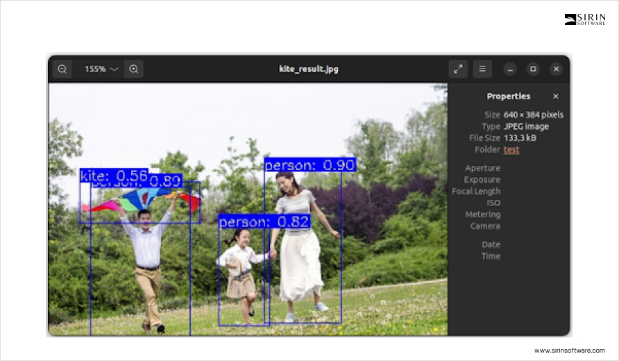
Detection results

We examined the detection results from running our neural network model, focusing on a key performance metric:

The Run graph execution time was 5.29743ms with an FPS of 188.77.

Before this step, we prepared by:

Scaling and Preparing the Source Picture: We used the cv2 library to preprocess the image to the required input format, which took about 400 milliseconds.
Loading and Preparing the Model: This step, which readied the model for processing, took approximately 40-42 seconds.
To enhance our analysis, we modified the C source code for more detailed metrics regarding the processing:
– Stopped saving the detection results to disk and displayed them on the screen instead.
– Set up the picture preprocessing to occur just once using the cv2 library.
– Loaded and initialized the YOLOv5 model once before processing it with NPU, doing this to avoid repetitive loading for each image processed.
– Processed the same picture 5 times to gather consistent performance data.
– Added additional messages with time markers to the source C code (markers like ‘–>’) and the Python script (markers like ‘—>>>’).
After these adjustments, we recompiled the code for NPU use and executed python3 yolov5_HW.py. The script’s execution included steps like starting the script, image preprocessing, initiating NPU processing, and detailed logging of each mapping phase. This provided a comprehensive view of the model execution, highlighting the efficiency of NPU processing.

When we recompiled the code to utilize the CPU for picture processing, we observed significant differences in processing times with the NPU’s superior performance.

sipeed@lpi4a:~/prj/test$ python3 yolov5_HW.py

—->>>Start script

Image preprocess (Python script), t=0.307

#Use NPU processing

–>Start time: 0.00033ms, input_num: 1

… [detailed mapping phase logs] …

–>Load and prepare tensors: 34912.26562ms

–>Init picture and tensors for processing: len-737280, path-./temp/image_preprocessed.bin, time: 39.97944ms

… [repeated picture processing logs] …

–>Detected objects are NOT written to the file!

–>Exit time: 0.06600ms

—->>>Total model(C code), t=35.186s

—->>>End script, t=0.0s

And CPU processing, which resulted in significantly longer processing times:

sipeed@lpi4a:~/prj/test$ python3 yolov5_HW.py

—->>>Start script

Image preprocess (Python script), t=0.307

#Use CPU processing

… [initial setup and processing logs] …

–>Processing time: 53360.99609ms (FPS=0.02)

… [repeated picture processing logs] …

–>Exit time: 1.96435ms

—->>>Total model(C code), t=266.897s

—->>>End script, t=0.0s

Results

Before diving into the main task of processing images with the NPU, we observed an initial setup phase. It takes roughly 35 seconds to prepare the NPU for use. This one-time setup step is unique to the NPU and wasn’t required when we processed images using the CPU.

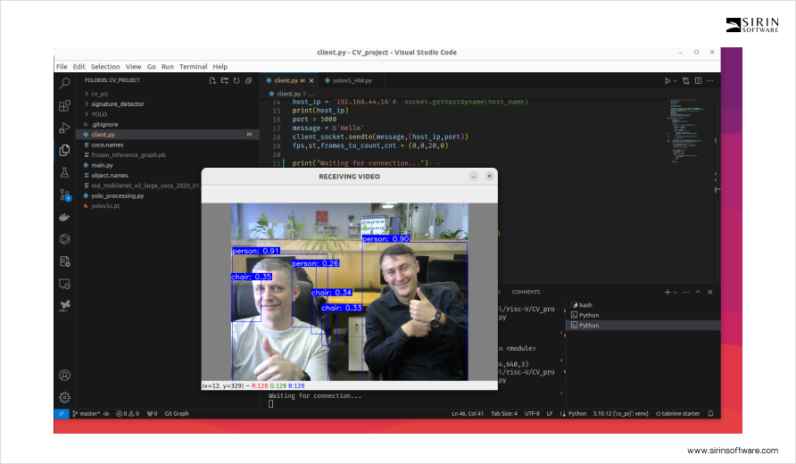
What should also be noted is a big difference in how fast images get processed between using the CPU and the NPU on the LicheePi 4A board. With the CPU, it’s pretty slow—only 0.02 frames per second (FPS), and it takes about 53,406 milliseconds to finish just one image. But when we switch to the NPU, things speed up a lot. We’re seeing speeds between 135 to 175 FPS, with each image taking just about 5 to 8 milliseconds to process.

Also, before we start detecting objects in the images, we need to get the images ready. This means making sure they’re in the right format for our model to work with. We tried two ways: one with a Python script and another with compiled C code, both using OpenCV. It turns out the compiled C code method is faster than using Python – about 1.5 times. We’re considering looking more into why this is the case.

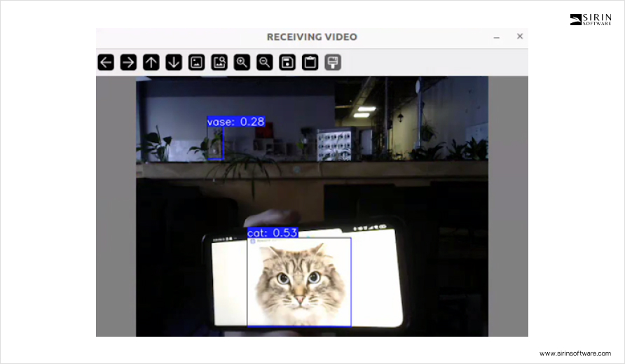
Conclusion

As we wrap up our discussion, it’s clear that the market’s growing availability of cost-effective hardware marks a significant step toward democratizing computer vision technology. These affordable yet powerful solutions open up opportunities for a wide range of businesses and innovators to integrate advanced vision capabilities into their projects without the steep costs. This shift makes CV more accessible and creates an environment where financial limitations are less of an obstacle to accessing this technology.

Yet, opening the full potential involves more than just acquiring the hardware. It requires a significant amount of expertise and knowledge. Here, the strategy of forging partnerships stands out as a viable alternative to developing an in-house team of specialists. Teaming up with external experts provides immediate access to the necessary skills and insights, smoothing the path to adopting these technologies. This approach accelerates the deployment process, diminishes the learning curve, and maximizes the advantages of cost-effective solutions.

Sirin Software: Your Guide to Computer Vision Tech

The benefits of utilizing custom solutions in CV are becoming increasingly apparent, offering a strong incentive to rethink our approaches to developing and deploying these technologies. For those ready to delve into how computer vision could revolutionize their operations, or for anyone looking for innovative solutions, the starting point is to clearly define your specific needs and explore the range of available options that can meet these requirements. This is where our team steps in as your ideal partner, ready to provide expert advice, support, or even a dedicated team to help you navigate through these options.

As we wrap up, it’s important to highlight our achievement in revolutionizing retail with AI-driven surveillance. For that task, we utilized the Rockchip RK3399Pro board and AWS cloud services to significantly improve security and customer insight in retail environments. Following the success of that project, we began questioning whether we could make computer vision technology even more affordable for wider use, and this is how the research, described in this article, was born.

We are eager to show you how our expertise can align with your ambitions, guiding you through the selection of affordable hardware solutions and beyond. Whether you’re interested in cloud-based, ready-made, or custom-built solutions, we are here to fit your vision and operational needs. Together, we can work towards making advanced visual technology smarter, more accessible, and fully achievable in any industry.